Something different on theSmallman today - actually something different all together. Since starting my Excel website and subsequent blog over 3 and a half years ago I have created over 300 pages from financial modelling to dashboard design to unlocking Excel's scripting dictionary. I have writen every word myself and have drawn extensively on my posts on Ozgrid and Chandoo forums. Today for the first time someone else is going to do the instructing. The two handsome gentleman above are Kasper and Mikel. They came to my attention through a Linkedin feed from Modeloff, the financial modelling world championships. They hail from Denmark - a place Australians feel a close connection with as one of our own is due to become Queen of Denmark one day. Kasper and Mikel have created an Excel blog which draws on their passion and knowledge of Microsoft Excel.

On Spreadsheeto - these gentleman have a bold ambition - "create the best information about Excel you have ever read." While this is an ambitious exercise, the guys have made a very strong start, posting countless useful blog posts on all things Excel. I wish them every success as they build their brand and Excel consulting business.

AUTO-HIGHLIGHT THE ACTIVE ROW WHEN A CELL IS SELECTED

In this guide, you will learn how to highlight a row automatically when you (or someone else) selects a cell in a sheet. This way it is always easy for the user to see which row is selected. This is helpful in spreadsheets that are set up with vertical entries – like a database. Be aware that this method requires some processing power, so if your file is already having trouble running smoothly, then this might not be a sustainable feature for you.

In this article and examples, I use Excel 2016 for Windows, but this method is also usable for you if you are running Excel 2007/2010/2013.

The General Idea

In order for this to work, we need two things:To set up a conditional formatting rule that highlights an entire row if a certain formula is true.Write a macro that recalculates the selected cell(s) when a new selection is made.These two things are fairly straightforward. I will show you how in the following.If you want to tag along as you progress in this guide, please download the project file here.

Highlighting rows with conditional formatting in itself is not difficult. It is the automatic part that is tricky. Check out this guide to conditional formatting if you are not up to speed with the fundamentals.

First, select all continuous data by selecting a cell in your data and using the shortcut ‘Ctrl + A’. In the project file, the selected range is A1:E55.

Then, click the ‘Conditional Formatting’-button on the ‘Home’ tab in the ribbon.

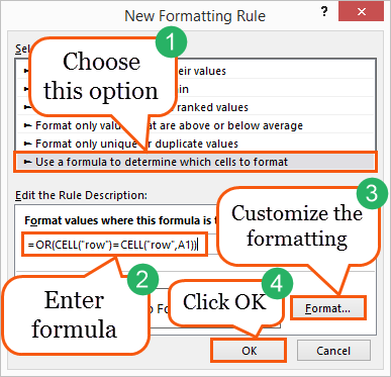
Click ‘New Rule’ and in the following dialog box choose ‘Use a formula to determine which cells to format’.

In the formula field, enter this formula:

=OR(CELL("row")=CELL("row",A1))

The last argument of the second ‘CELL’-function (the A1) must be the top left cell of the selected data (from before you clicked the ‘Conditional Formatting’ button).

Customizing the Format

It is up to you whether the row is highlighted by bolding the font, changing the fill color or something entirely different. A word of advice, though: Please don’t make the row stand out too much. If you color the row blood-red people will have a difficult time reading the values in the row. It will then be tiresome and hard to find the corresponding values in the sheet, which goes against the original purpose of the feature.

Customize your format by clicking the ‘Format…’ button in the ‘New Formatting Rule’ dialog box.

From the tabs at the top of the dialog box, choose which kind of formatting you want to apply. For this example, I have chosen a yellow fill for the cells in the row. Then click ‘OK’.

Writing the Macro

I have written the macro for you, but it is not complicated. It simply looks like this:

Option Explicit

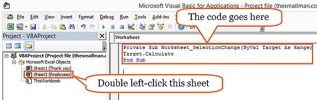
Private Sub Worksheet_SelectionChange(ByVal Target As Range)
Target.Calculate
End Sub

This code goes not in a normal module, but in the code belonging to a specific worksheet. Use the shortcut ‘Alt + F11’ to get to the ‘VBA editor’.

Double click ‘Sheet2(Employees)’ in the ‘Project Explorer’ and paste the code from above. If your ‘Project Explorer’ (the menu to the left) is missing and it does not look like the screenshot on your computer, you need to toggle on the ‘Project Explorer’. Click ‘View’ in the menu and click ‘Project Explorer’.

Conclusion

There you have it. Setting this up is quite easy and quick to do, but adds a nice touch to the system you have created if it holds data in a database form. Test it out for yourself.