
Power Pivot - A User Guide
Power Pivot has been a blessing in the world of data analysis, manipulation and reporting. This article will look a real world example of loading data, making power pivot connections and using power pivot (pivot tables) to report data in Excel. The tables will lead into an eye catching PowerPivot report complete with slicer which will enable us to consolidate the report with a slicer.
Increasingly organisations are having to deal with the management of bigger datasets. The associations, clusters, trends, differences or anything else that might be of interest to you will likely have to be gleaned from large datasets and this would normally require tons of VLOOKUP, SUMIFS, and/or array formulas to produce a cohesive analysis. These things tend to bring "native" Excel to its knees even with tens of thousands of rows, much less hundreds of thousands. But, and it is a big BUT, Microsoft has created PowerPivot –10 years ago!
The Power Pivot Exercise
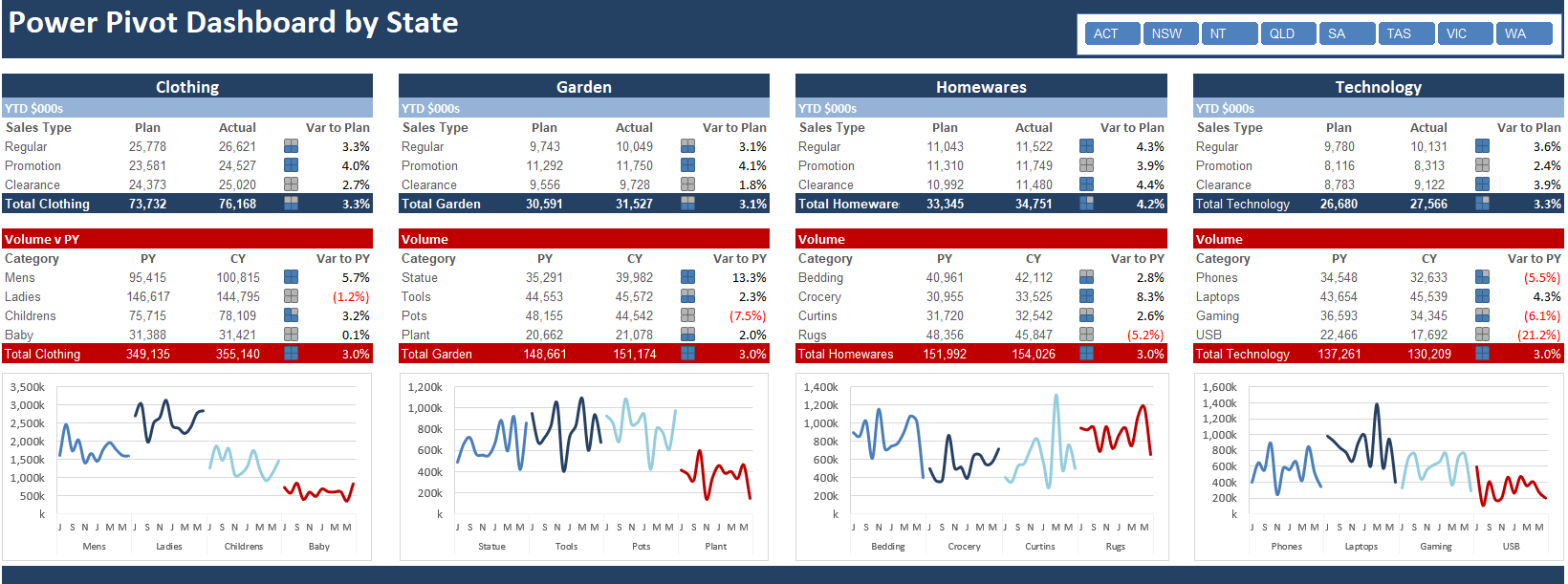
The data we are going to analyse is a typical data set which compares many tables. The primary PowerPIvot data sets are the current year and the prior year’s data tables. There will be a range of PowerPivot support tables. The data is reasonable in terms of its size with the prior year data being 35,000 rows and current year to date being 36,000 rows. The data is stored in a range of data tables and the task will be to join the tables and compare last year’s data with this year’s data. The final result will be as follows.
We will gather our data from 3 sources – An Excel file containing the fact (lookup data) and transnational data for the current year and an Excel database containing prior year’s transnational data. The import will involve the update from these two data sources.
Extracting PowerPivot Data
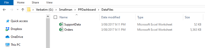
There are 3 files to download which can be found below. The file where the data is to be incorporated is called PowerPivotDashboardStart. The other two files will feed into this one. The import will involve the update from these two data sources. The Lookup file has all of the lookup tables and the data file has the raw transactional data in it.
Upload the files and we can begin the PowerPivot tutorial.
Loading Data with PowerPivot
Starting with the Dashboad start file we want to load the data into this file. Loading data is how the information gets from the web, a text file, an Access database, a spreadsheet or your ERP system, into the PowerPivot engine where we can manipulate the data.
Using the PowerPivotDashboardStart.xlsx file - On the Power Pivot menu:
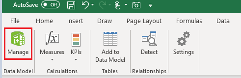
On the PowerPivot Menu - choose Manage.
By clicking Manage - you will be taken into PowerPivot.

Choose From Other Sources.
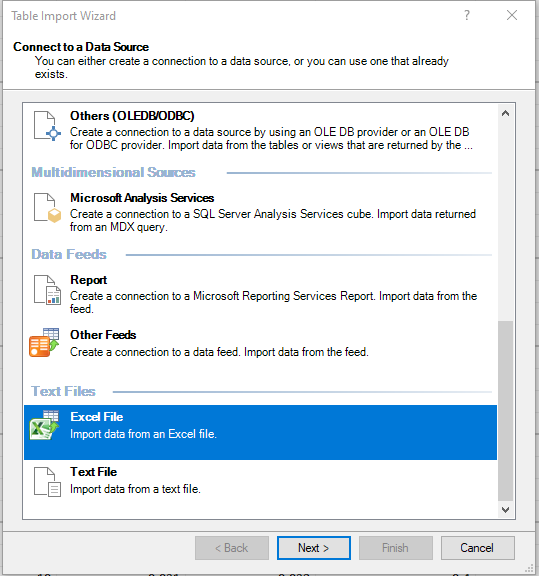
Towards the bottom of the form is a Excel File option. Use that to select the files that will be required. Choose Next.
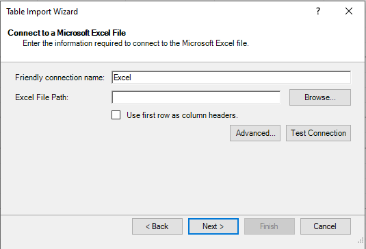
Before clicking the browse button click Use first row as column headers - this will save you the trouble of forgetting later. I have got in the habit of pressing this first as I have missed it far more times than I care to remember.
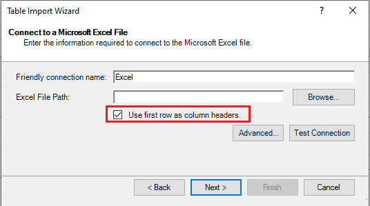
After this check box is ticked click the browse button and browse to the files location.
Choose Support Data.
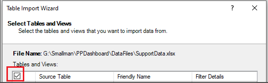
By ticking the above check box all of the items in the list are selected.
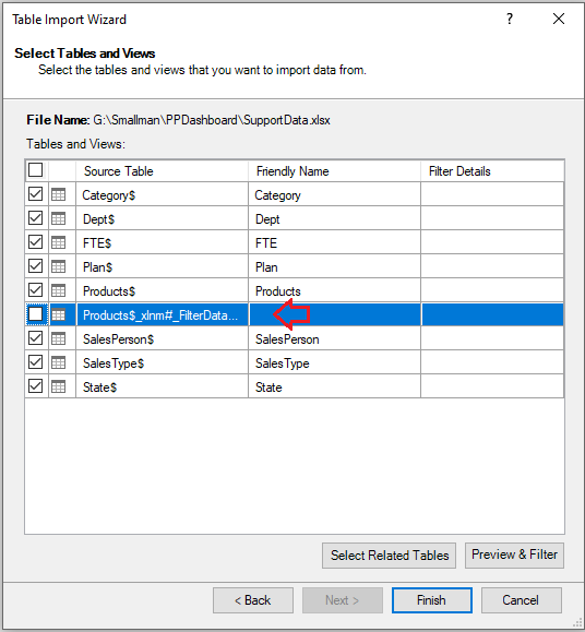
Tick the Source Table check box - then untick the Products_xlnm line. This is a throwback to a table which ones lived in the file over the products data. This will duplicate the Products table if left unchecked.
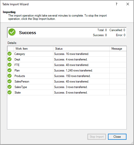
If everything loads correctly the above is what you should see - with the PowerPivot wizard displaying no errors.
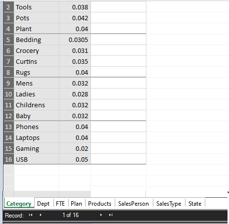
Just like tabs in an Excel workbook you should see the tables loaded into PowerPivot.
Follow the same process with the Orders Excel file.
Skip to the load section.
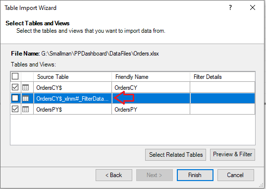
Be sure to un-tick the xlnm table as this only serves to duplicate the table in PowerPivot.
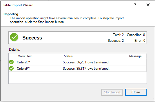
The above tables should load into PowerPivot - click the close button.
All of the tables are now uploaded into PowerPivot.
Joining Data Tables in PowerPivot
The tables need to have a common link so anything which is going to be reported on needs a small table which is used to link the two tables together effectively creating a many to 1 relationship. The (1) in the many to 1 comes from the Lookup table where there is 1 instance of the unique identifier and the many comes from the transnational table. For example:
Jan, Feb, Mar
These might be the unique month names in the lookup table entitled (Date), the key is they only appear once in the lookup table. However, in a larger transnational table there will be multiple instances of the month. By funnelling the data through a smaller table Excel understands the join.
Many to 1 Relationships
In order for PowerPivot to create a join, there needs first to be a many to 1 relationship as explained above. So in the following example the State table has one instance of each State while the Plan table has many instances of the State. The join is created by dragging and dropping State from either table and dropping it over the top as denoted by the green area that appears.
Once the many to one join is created - PowerPivot creates the join type signifying the many (*) and the 1 with a join line and the wildcard symbol and the number 1.
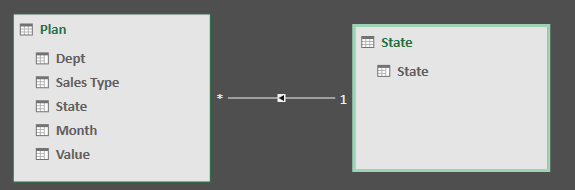
You can see above how the 1 is closest to the State table - this denotes the State as the one table in the many to 1 relationship and conversely that wildcard symbol is next to the Plan table denoting this table as the Many table.
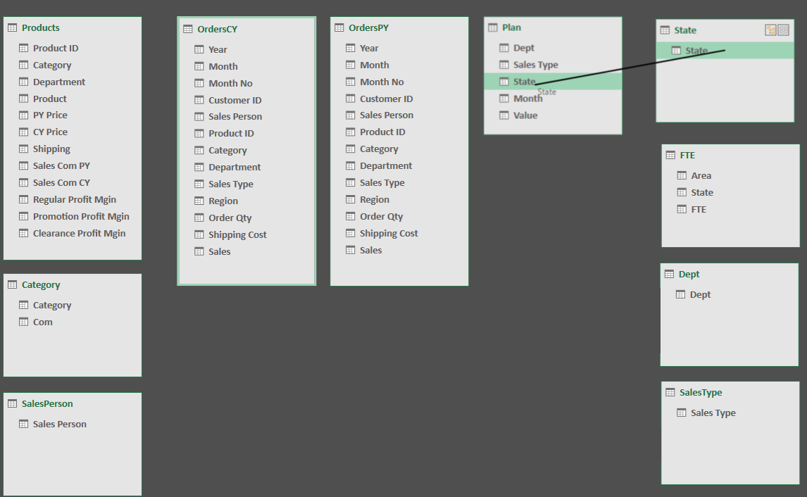
There are 4 joins for State, in the OrdersCY and Orders PY
Orders Tables
State = Region
FTE Table
State = State
Why have I not created a field in the Orders table called State - simple, in the real world data coming from different systems have different names. So too in this real world example the field names are different. This should tell you that fields of different names can be joined as long as the data inside the fields is the same and it is not easy to get data that marries neatly from multiple systems you have no say in designing.
Other PowerPivot Joins
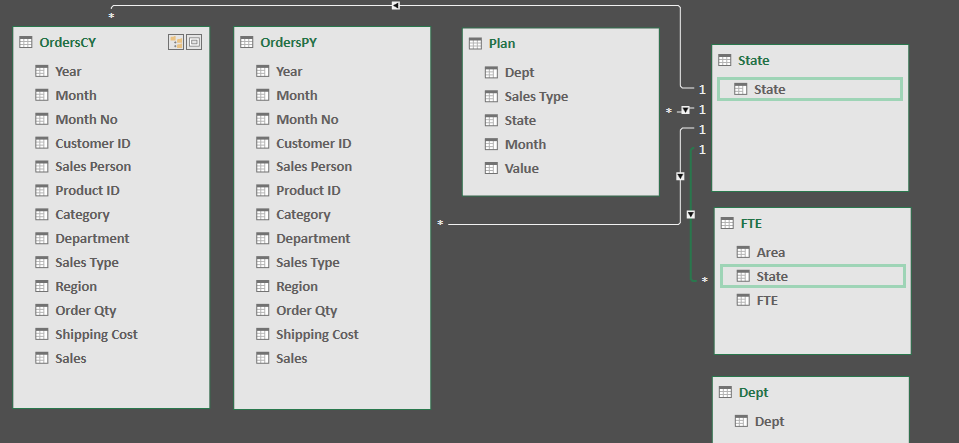
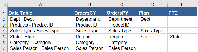
There are 16 joins in all and there should be 16 arrows on the screen. This should complete the linking exercise. The joins are as follows;
When the data is successfully joined in PowerPivot the table looks similar to the below.

The T is for Transaction table - these go towards the centre of the set up. The L stands for Lookup. These go around the outside of the transaction tables. The lookup tables feed into the transaction tables.
It might be a little daunting but just take it one step at a time and you will create all the joins.
When PowerPivot Joins are Incorrect
If you happen to make an incorrect join when joining the tables - this is easily corrected.
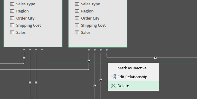
Right click the relationship you wish to delete and choose Delete.
Generating the Pivot Tables
Now that the joins are created we can go ahead and make the pivot tables which will make up the bulk of our PowerPivot output report. Regular Pivot tables generally have one data source, though pivot tables can be made from multiple sources this is not common.
On the home menu there is a Pivot Table button.
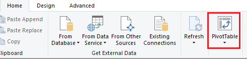
Depress the button and you will be taken into Excel to set up the pivot tables.
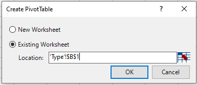
When asked where you want to place the Pivot Table - choose B1 of the Type tab.
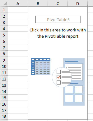
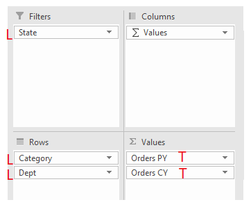
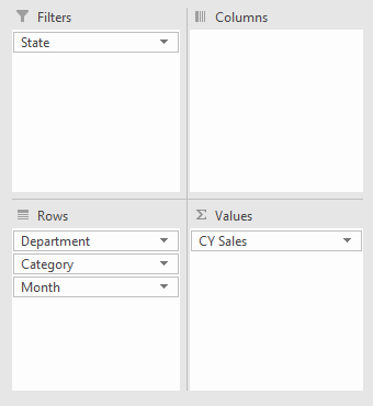
A blank Pivot Table icon will appear. In the field settings on the right - choose State
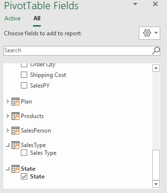
Choose the Lookup table State and put that as the report Filter.
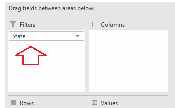
Place the State in the Filters section.
The L in front of the field setting table is the type of table you should choose the data from, eg State comes from the lookup table called State. Don’t…..don’t…..don’t choose your fields from the transaction tables OrdersCY and OrdersPY. I can not stress this strongly enough.
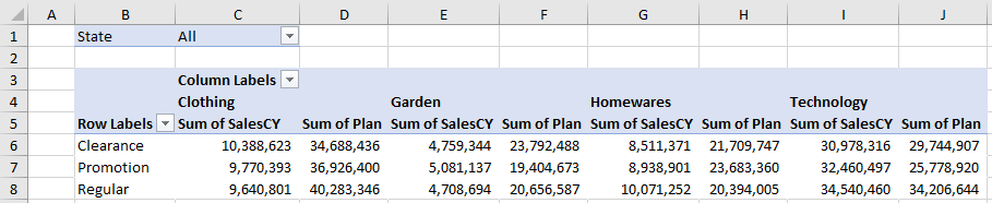
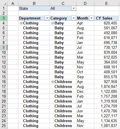
The above is how the pivot table should look when all of the fields has all of the information in it.
PowerPivot Progress
The above data is enough to populate the top third of the PowerPivot dashboard.
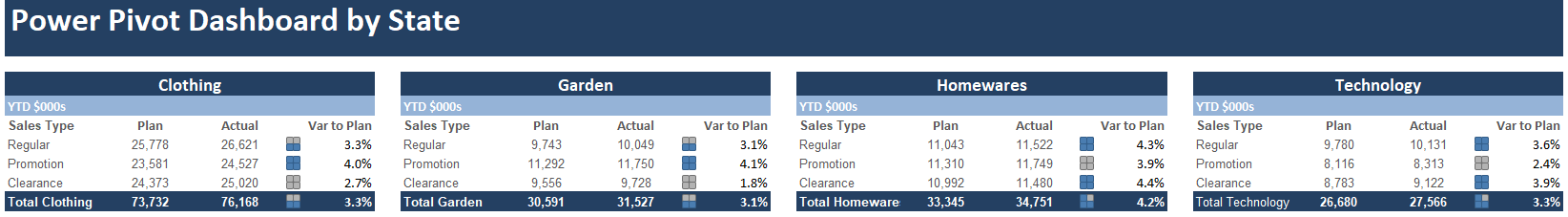
The data can be corralled into the above format.
Make a copy of the original dashboard and paste it onto the category sheet.
Summary by Category
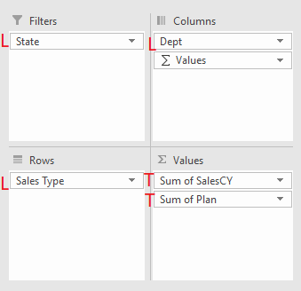
The following is the setup for the Pivot table.
The State, Category and Dept needs to come from the lookup tables. The orders are from the PY and CY tables.
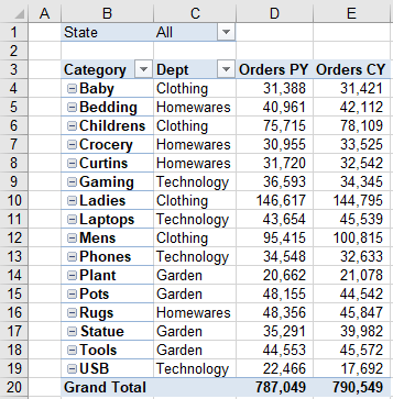
The above is the way the data can be structured.
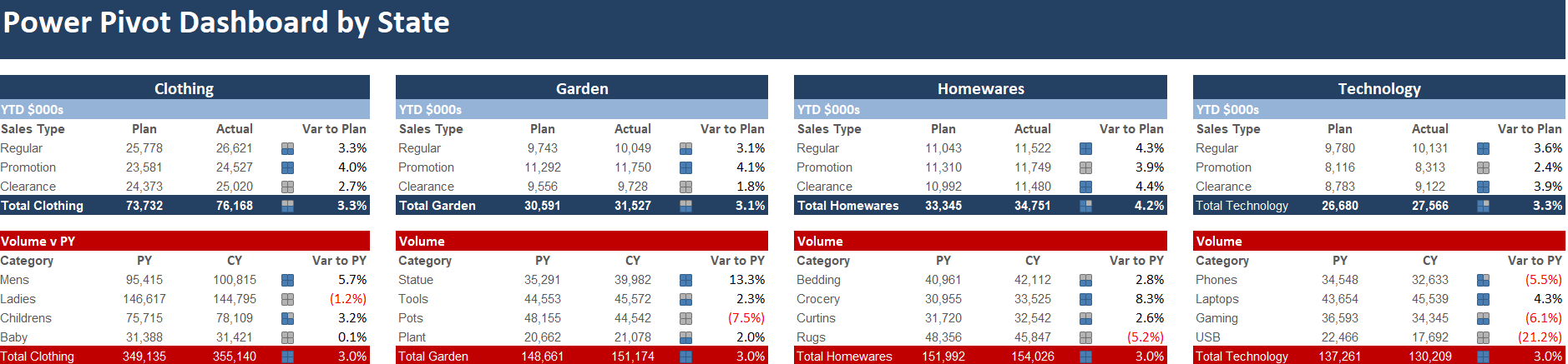
The pivot table above can feed the red areas above. The first two pivot tables account for the majority of the dashboard.
Populating the Dashboard Charts
The charts in the PowerPivot report will be extracted from a single power pivot table. The data will need to be added in the following format to draw that information out.
Be sure to use the Lookup State however all of the Orders CY data can be used for the rest of the pivot table.
The table will need to look as follows.
The charts can be added by taking the data from the table above. That is all that is required to complete the model.