
The SUMPRODUCT Excel Function
The SUMPRODUCT Excel Function is one of the most important Excel formulas to master. It is rightly one of the most powerful and versatile formulas in the Excel arsenal of formulas. In Excel SUMPRODUCT will multiply the corresponding elements of a range which meet a specified condition and then return the sum of all the products.
The following video outlines the details in this article. The following Excel file will help you follow along with the SUMPRODUCT lesson.
The SUMPRODUCT Syntax:
=SUMPRODUCT(Array1,Array2,Array3…)
Putting the above into context I tend to look at the syntax a little differently. Let’s use a two criteria formula as an example of how to lay the SUMPRODUCT out.
SUMPRODUCT ((Criteria Range 1 = Criteria 1) * (Criteria Range 2 = Criteria 2) * (Sum Range))
The Above is a 2 criteria SUMPRODUCT formula which is the way my mind lays out a typical SUMPRODUCT calculation. Start the SUMPRODUCT formula with 2 brackets, the first criteria range will have the first criteria sprinkled throughout from 1 to many times. The multiplication sign joins the first criteria with the second. The second criteria range will have the second criteria sprinkled throughout from 1 to many times. Finally the SUM range is the range which needs to be calculated based on the two criteria.
Behind the scenes this is happening. Let’s use a simple Example.
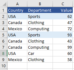
We have countries and we have departments. Let’s say we want to sum all of the instances of USA and Sports.
=SUMPRODUCT((A2:A10=E2)*(B2:B10=F2)*(C2:C10))
The above will return a result based on data in Column A being equal to USA, Column B being equal to Sports and the numerical values in Column C will to added together.
Behind the scenes the SUMPRODUCT formula will produce the following results for column A.
{1,0,0,1,0,0,1,0,0}
The second criteria in Column B will be as follows:
{1,0,0,1,0,0,0,0,0}
And the calculation for the three matches will be as follows:
(1 X 1) X 62 = 1 X 62 = 62
(1 X 1) X 62 = 1 X 93 = 93
(1 X 0) X 60 = 0 X 60 = 0
The final equation is:
62 + 93 + 0 = 155
All of the other equations will produce the same zero. Any part of the equation which does not match produces a zero, so in the third example the Department is CAR and it is excluded as CAR is equal to zero or FALSE for a match. SUMPRODUCT produces a series to TRUE results ones and FALSE results zeros to generate the equation. The ones (1) are matches the zeros (0) are not.
The output of the formula can be seen below.

NOTE: Try and create formula so it covers one cell past row of data, that way when you INSERT COPIED CELLS, your formulas will adjust accordingly without being manipulated.
The above is a little simplistic though as the SUMPRODUCT formula is way more powerful. When we want to consider multiple columns to SUM at once, the SUMPRODUCT formula comes to the front of class.
Extending the SUMPRODUCT Function
Once the SUMPRODUCT function is extended the formula itself comes into its own and the genuine power of SUMPRODUCT is unleashed. The SUMPRODUCT formula has the power to sum across multiple columns. It can Sum a single column amongst many or it can consolidate many columns of numerical data. It is quite simply other worldly in its powers.
Let’s have a look at the following addition to our problem. We will add quarters and extract the summary of a particular quarter.
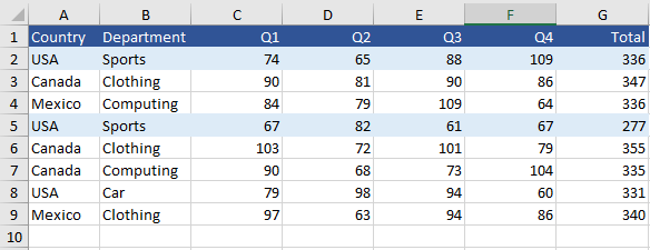
We will keep the criteria the same – so let’s look for USA and Sports but let’s add Q2 for quarter 2 to the analysis. Which means we want to consolidate data based on 3 criteria.
=SUMPRODUCT((A2:A10=I2)*(B2:B10=J2)*(C1:F1=K2)*(C2:F10))
The section in bold is the addition. We add the column references and the criteria, also the Sum range needs to expand to cover the columns in the criteria range.
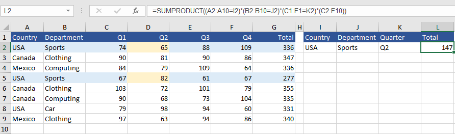
The two numbers which need to consolidate are 65 and 82 (Cells D2 and D5) these are the only two cells that meet the above criteria (USA, Sports, Q2).
SUMPRODUCT to Sum Multiple Columns
Lets’ take the concept to the next level where SUMPRODUCT is asked to perform consolidations over multiple columns. This is where SUMPRODUCT is king. It has the capacity to use operators to gather the sum of more columns. Let’s looks at the following data set.
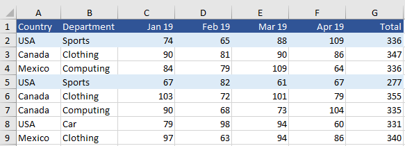
The data now has months running along the top. We can summarise the data up to and including a date with the help of operators. If we want the sum of all of the columns up to March the Less than or equal to sign (<=) can be used.
=SUMPRODUCT((A2:A10=I2)*(B2:B10=J2)*(C1:F1<=K2)*(C2:F10))
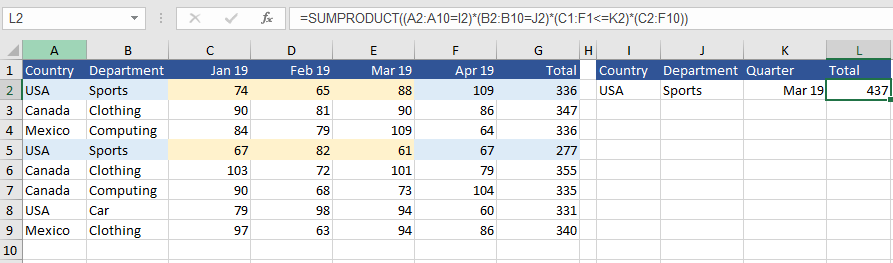
It is worth noting that the dates are literal dates and not text. As dates appear as numbers SUMPRODUCT allows them to be consolidated seamlessly with the help of the operator less than or equal to.
The following Excel files shows the SUMPRODUCT examples above:
