
INDEX AND MATCH Formula
The INDEX AND MATCH combination are a very powerful tool in the Excel world. After the VLOOKUP formula it is probably the most used lookup formula. The INDEX and MATCH is used in a whole range of situations to return data left right up or down, it has a flexibility to it that makes it extremely useful.
The following video goes through the practicalities of INDEX and MATCH in this page. The following file goes with the attached Youtube video.
The INDEX and MATCH formula is not as heavily used in Excel because it is a nested formula, a combination and I guess users find the process a little more long winded or confusing. If you do manage to work your head around INDEX MATCH your ability to return data will be vastly improved over the VLOOKUP formula which is limited to looking up data to the right of the unique identifier.
This article takes you through a range of examples where Excel’s INDEX and MATCH can help you lookup data in different ways. Let’s first split the two functions to see what they are both doing and see how together they make the perfect marriage of convenience.
The INDEX formula
INDEX is the key behind the combo and it is remarkably simple. The premise for the INDEX formula is it returns text or value within a range of values that meet certain location criteria.
The syntax is as follows:
=INDEX(Range, Row offset, Column Offset)
Using the Row offset as an example here is a very simple use of the INDEX formula.
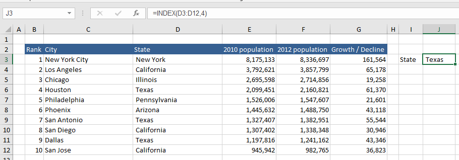
Above we have a set of cities and the idea is to choose one of the cities. The state of Texas is the 4th item in the vertical list of cities. New York, California, Chicago, Texas. So to use the INDEX formula we first isolate the cities in the vertical range.
=INDEX( D3:D12,
The second part of the formula is to look for the Row number. As Texas is the forth item in the list a hard coded 4 is used as the ROW reference.
=INDEX( D3:D12, 4)
That is all there is to it. We don’t need to use the column reference as we are just looking in a single column.
NOTE - only row reference is required if you don’t need the column.
What if we need a 2 Dimensional Reference
Using the column in the above example to return the population for Texas in say 2010 is a matter of extending the range to cover more of the table and retuning the relevant column. If we change the formula as follows:
=INDEX( D3:G12, 4, 2)
If we expand the reference for the table from Column D to include column G then we have a good portion of the table mapped.
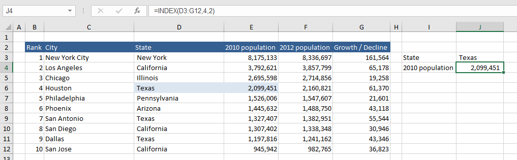
Now we are incorporating the column reference to return the population. Above 2010 population is column E and the reference starts in column D, so D is column 1 and E is column 2 in the range selected.
Using the Match Formula
The Match formula returns the row or column reference (A number) based on a set of criteria. For example we may search for the term Texas in the example given in Column D. It will return the number 4. The syntax for the MATCH formula is as follows:
MATCH( Lookup Reference, Lookup Range , Match Type)
The Lookup Reference is the cell being searched for.
The Lookup Range is the Range where that text or value is contained within.
Match Type - The number -1, 0, or 1. The match_type part of the formula specifies how Excel matches lookup reference with values in lookup Range. The default value for this part of the formula is 1. However, mostly this formula is used with the Value 0 so if you want an exact match it is highly advisable to type zero (0) as a habit.
So the MATCH formula would therefore be:
=MATCH( J3,D3:D12,0)
The result will be the number 4. This is a pivotal point as 4 was the Row reference we were searching for in the INDEX formula. Now the juices are flowing. The following is what is happening in the formula above.
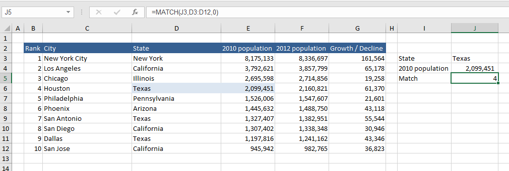
In text form this is what is happening:
=Match(“Texas”, Range D3:D12, 0 Exact Match)
So taking this back to the nature of the article - the INDEX and MATCH can be combined in a nested formula that covers off both the INDEX (the range the States are stored) and the Match for the Row reference of the appropriate State.
INDEX AND MATCH Combined
Taking the concept back to the premise of the article you should now be able to see how we can use the INDEX formula to outline the range the state is in and the MATCH formula to trap the ROW reference for the state. With these two nested formula we can trap the 2010 population for Texas without a hard coded ROW value.
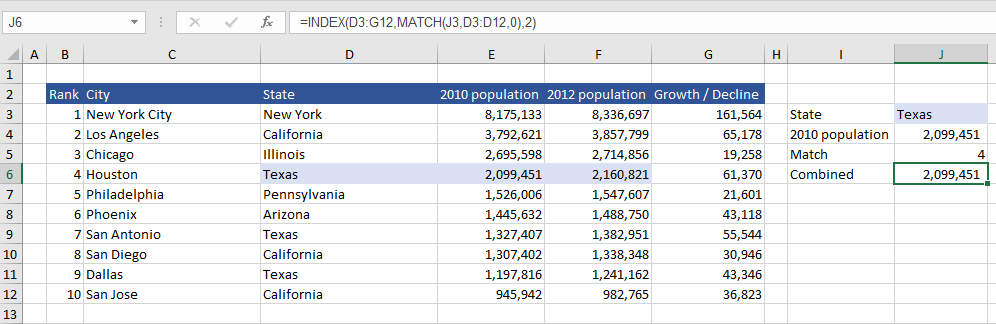
The formula above looks like the following:
=INDEX(D3:G12,MATCH(J3,D3:D12,0),2)
Where D3 to G12 is the Range we are examining and MATCH comes to the party to help solve the row for Texas.
March( J3 - the cell Texas is in (blue above)
D3 to D12 - the cells the States are in.
0 - for an exact match of the state name.
2 - this is the Column reference and it is a reference to Column E.
It is a bit sad that the column reference is hard coded in this Example so we can weaponise the formula by nesting a further MATCH formula inside the INDEX formula to return any column that relates to the Texas state.
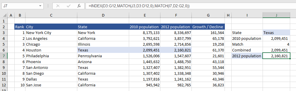
The formula in full above is as follows.
=INDEX(D3:G12,MATCH(J3,D3:D12,0),MATCH(I7,D2:G2,0))
For ease I have been not adding references so in practical terms this is how the formula would be written with correct referencing.
=INDEX($D$3:$G$12,MATCH($J3,$D$3:$D$12,0),MATCH($I7,$D$2:$G$2,0))
I hope the article helps build your understanding of the INDEX and MATCH formula. The following is a file with the above examples of INDEX and MATCH.