
INDEX Formula in Excel
The Excel INDEX formula is designed to return a single text or numerical value from a range. INDEX is used to return the row or column or both inside of a given range. To add increased flexibility to the formula INDEX is regularly used in conjunction with the MATCH function, where the MATCH function generates the row/column position to retrieve for the INDEX formula. The two formulas are a perfect match for one another.
The following is a brief video on the use of the Index formula in Excel. Use the file at the below to follow along.
The INDEX formula is t he perfect location based formula. You put a range to evaluate and tell it the Row and Column coordinates and INDEX goes to work to return the value in the specified location.
The syntax for the INDEX formula is as follows:
INDEX(Range, Row Reference, [Column Reference])
The Range is the area which contains the values you are evaluating.
The Row Reference is the Row from the top of the range, this is a number.
The Column Reference is the Columns from the start of the range, this is a number.
Let’s have a look at a practical example.
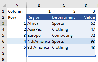
The formula to extract the value 93 in blue above is as follows:
=INDEX(B3:D8,4,3)
Where B3:D7 is the range being evaluated. The ROW reference is 4, and the column reference is 3 as it is the third column.
It is worth noting that the INDEX formula can be used with the row reference or the column reference or both. For example f you are sure that column 3 is the one you wish to evaluate the following can be simplified to just look for the ROW reference. The formula becomes:
=INDEX(D3:D8,4)
Notice the range is shortened to just include Column D. As the dataset is a single column the ROW is the only reference point required in the INDEX formula.
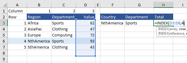
When D becomes the column of focus (D3:D8) then the only thing to evaluate is the row number.
Further Reading: