Excel SUMIF Formula

The SUMIF formula sums all of the cells that meets a condition or criteria.  The SUMIF function will work nicely with logical operators such as greater than > less than < does not equal <> is equal, wildcards * ? for partial cell matching.  This article explains the logic of the SUMIF formula with some practical examples.

SUMIF with Text Criteria

The SUMIF formula can be used to sum how many cells in a range of cells meet a given condition.  Let’s say we have a list of countries in Column A and we want to Sum how many countries are USA and return the sales.  Firstly the range that contains the countries and the criteria in the above example would be “USA” or a direct cell reference to USA.  The following will show both methods. 

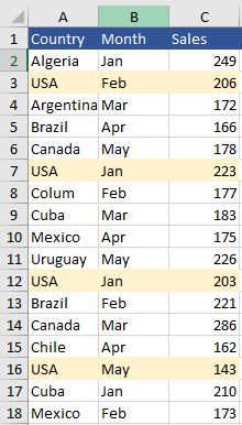
The above is a sample of countries that has the USA several times in the range.  Our task is to SUM the amount of times that USA appears in the range specified.  The Syntax for the SUMIF formula is as follows:

=SUMIF ( Criteria Range, Criteria, Sum Range)

Firstly the range that contains the countries and the criteria in the above example would be “USA” or a direct cell reference to USA.  The following will show both methods.  Firstly the direct cell reference as this is better practice. 

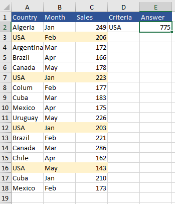
The SUMIF formula becomes:

=SUMIF(A2:A19,D2,C2:C19)

Next let’s look at what to do if we need to add a direct reference inside a formula.

=SUMIF(A2:A19,"USA",C2:C19)

Notice that USA is in double quotation marks “USA”.  Where possible it is better to refer directly to a cell reference rather than hard coding the country in a formula.

Extending the SUMIF Formula

If we want to check the dataset for values that are greater than a given month in our data.  We can place the operator in the cell or we can hard code the operator in the formula and refer to the cell with the value.  Let’s say we want to SUM if the month column is greater than or equal to Feb.

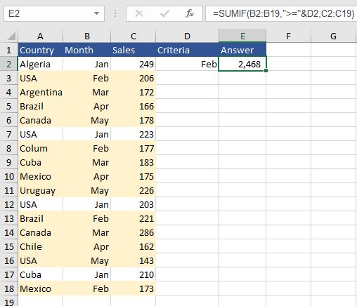
The coloured cells are those included in the SUM. Others, which are January, are excluded.  It is worth noting that the Months columns are actual Dates not text.  It always works better in Excel if we use Dates rather than text to represent dates.  The syntax becomes:

=SUMIF(B2:B19,">="&D2,C2:C19)

You will notice the greater than or equal to sign in double quotation marks “>=” this is then joined together with the ampersand sign & with the cell reference in  D2.

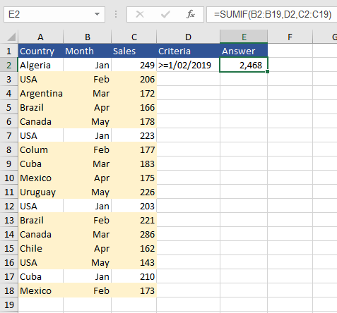
While including the greater than and equal sign in the cell itself keeps the formula a little simpler. 

=SUMIF(B2:B19,D2,C2:C19)

It keeps the formula tight but people might have trouble reading the criteria.

SUMIF with Question Mark

Using the USA example the following will SUM for any characters after the first character.  Note – the question mark works one character at a time so it will check for S and A but needs 2 question marks.

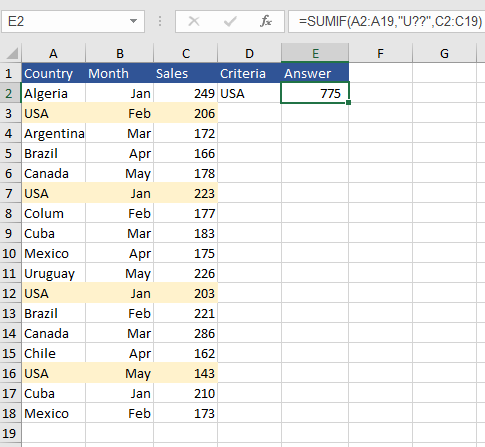
The formula becomes:

=SUMIF(A2:A19,"U??",C2:C19)

Notice the two question marks ??, these represent the S and the A but will also work for any other letter.

SUMIF with Wildcard

Let’s use the wildcard character * to SUM all of the countries starting with US in the list.  The formula works by including the letters US followed by the wildcard character * in the formula.

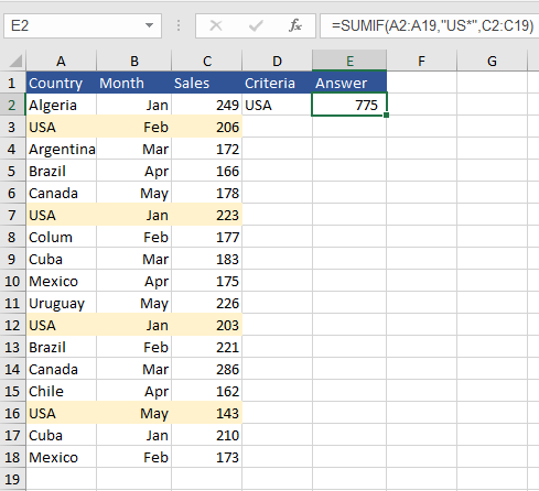
The formula becomes:

=SUMIF(A2:A19,"US*",C2:C19)

Notice the US and wildcard character are all in quotation marks “US*”.

The following file contains the examples in this lesson.  Remember practice helps.