
Conditional Formatting Traffic Light Effect
Conditional Formatting showing a traffic light effect can be a very handy tool for Excel data which relates to information which is date critical. In the following Excel file I will look at data which is 7 days overdue (Red), 2 days or greater overdue (Yellow) and less than 2 days overdue (green). The following is the Excel conditional formatting rule for each of these.
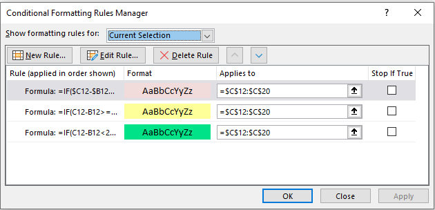
Red =IF($C12-$B12>=7,1,0)
Yellow =IF(C12-B12>=2,1,0)
Green =IF(C12-B12<2,1,0)
In the Conditional Formatting Window the Excel formulas should look similar to this.
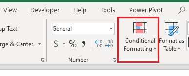
On the Home menu - choose Conditional Formatting;
Now Choose Use a formula to determine which cells to format.
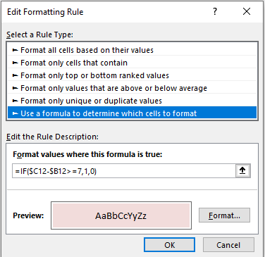
Enter the formula into the format box.
The following is an example of the the above.
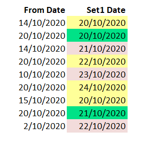
The following Excel files shows the workings from the above.