USING THE EXCEL VLOOKUP FUNCTION

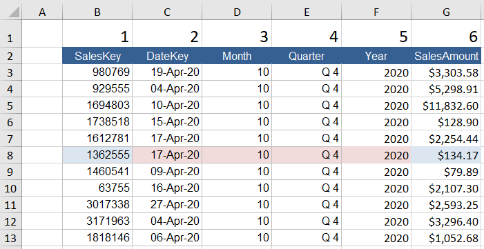
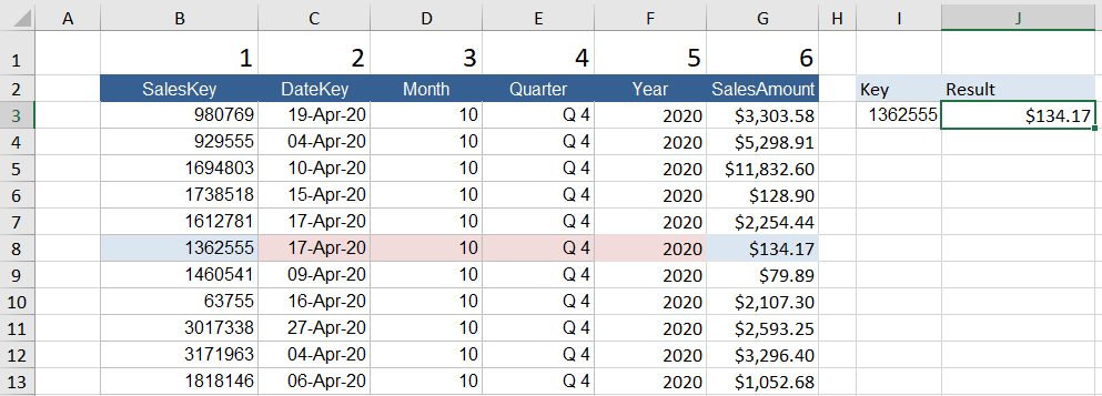
VLOOKUP is an Excel function which allows you to lookup unique data. The premise is to look for a unique identifier in the first column and return data in the same row in another column. The Excel VLOOKUP which is short for vertical lookup, would have to be one of the most used Excel functions.

The following Youtube video is an outline of the lesson below. Use the following file to follow along.


VLOOKUP Arguments


The VLOOKUP syntax has four arguments.

=VLOOKUP (Lookup Value, Range, No Cols Offset, True/False)

Reference - the cell or text or value you are looking.

Range- the range that reference is in contained within. The Reference must be contained in the very first column as the data is looked up from left to right.

No Cols Offset - from the reference column

True/False -This is the type of match - either exact or approximate.

Key Point - VLOOKUP Only Looks To The Right!

VLOOKUP has two arguments for matching data, exact match and approximate match. The choice for either of the two is made with the 4th argument. It is True False above but Excel calls this [Range Lookup]. We put a False (or zero) to make Excel get an exact match or True (or One) for an approximate match.

Example 1 - The VLOOKUP Exact Match

Probably the most well known and used method for VLOOKUP is the exact match. This type of match with the VLOOKUP is ideal when you are looking up a unique key and want to return data based on that key. The following table shows the sales key and if you are looking for the sales key the VLOOKUP can return all the columns to the right.

 
Vlookup formula excel
 

Once you have identified your unique identifier (SalesKey above) you can use VLOOKUP for any column to the RIGHT of the column you are searching for.

The column Offset is 6 columns remembering to include the first column in your count.

 
VLOOKUP FORMULA
 

The syntax to a lookup for the above would look like the following.

=VLOOKUP(H2,$A$2:$F$10,6,FALSE)

 
VLOOKUP
 

Where H2 is the Lookup value 1362555, the Range Lookup is A2:F10, the column offset is 6 and the type of lookup is an Exact lookup FALSE (this can also be 0 - which is the method I prefer). The fourth argument of the VLOOKUP will return an NA error if the function does not find the lookup value (SalesKey) in the above example.

To return the year for the VLOOKUP the only thing we would change would be the Column reference. This would be 5.


=VLOOKUP(H5,$A$2:$F$10,5,FALSE)


VLOOKUP will work on any of the columns to the right of the first instance of the SalesKey above. It is important to remember with VLOOKUP that if your lookup key is not unique the first instance in the list starting from the top will be returned. The other instances will not be considered.


Multiple Instance of a Match

What if there are multiple instances of a match with VLOOKUP - in this instance the VLOOKUP will pick up the first instance from the top down. When VLOOKUP finds the first match it will return the result.

 
VLOOKUP fist match
 

In the above example there are two instances of the sales key. The VLOOKUP will start in row 3 and go down column B till it finds the first instance of the saleskey 929555 and it will return the first sales amount assuming the following VLOOKUP formula.

=VLOOKUP(H2,$A$2:$F$10,6,FALSE)

The result of the VLOOKUP will be $5,298.91 as this is the first instance of the SalesKey. If you want to sum both instances of the SalesKey then you need a different formula and perhaps SUMIFS or SUMPRODUCT is the formula for this situation (SUMIFS is the better solution).

Example 2 - The VLOOKUP Approximate Match

The approximate match with VLOOKUP is not used as commonly, however is exceptionally useful. This type of VLOOKUP provides the opportunity to group data and search within bands for a particular result. One such example is grades in school, where grades are given inside certain scores. From 60-75 might be considered a C grade.

Vlookup true criteria

The formula is C2 is as follows:

=VLOOKUP(B2,$E$2:$F$6,2,TRUE)

Where B2 is the score, E2:F6 is the range of the tables with the banded grades, 2 is the column to offset by and TRUE (or 1) is for the last argument which is for an approximate match. Using the VLOOKUP formula avoids multiple IF statements which I still see a lot today. VLOOKUP gets a lot done with a small amount of text. Use it wisely.

The following Excel file can be used to practice the VLOOKUP technique and goes with the above video.

VLOOKUP.XLSX