
USING THE EXCEL HLOOKUP FUNCTION
HLOOKUP is a function which allows you to lookup unique data in a top down approach. The premise is to look for a unique identifier in the first row and return data in the same column in another row. The Excel HLOOKUP which is short for horizontal lookup, is not used as much as VLOOKUP however it is exceptionally useful.
The following is an instructional video on how to create a HLOOKUP formula. The following file goes with the Youtube video.

The HLOOKUP syntax has four arguments.
=HLOOKUP (Lookup Value, Range, Number of Rows Offset, True/False)
Lookup Value - the cell or text or value you are looking.
Range - the range that reference is in contained within. The Reference must be contained in the very first Row as the data is looked up from top to bottom, so row based.
Number of Rows Offset - from the reference row (the first row)
True/False -This is the type of match - either exact or approximate.
Key Point - HLOOKUP Only Looks down ways
HLOOKUP has two arguments for matching data, exact match and approximate match. The choice for either of the two is made with the 4th argument. It is True False above but Excel calls this [Range Lookup]. We put a False (or zero) to make Excel get an exact match or True (or One) for an approximate match. If no match is found with the FALSE argument - an NA is returned. This tells you there is a problem.
Example - The HLOOKUP Exact Match
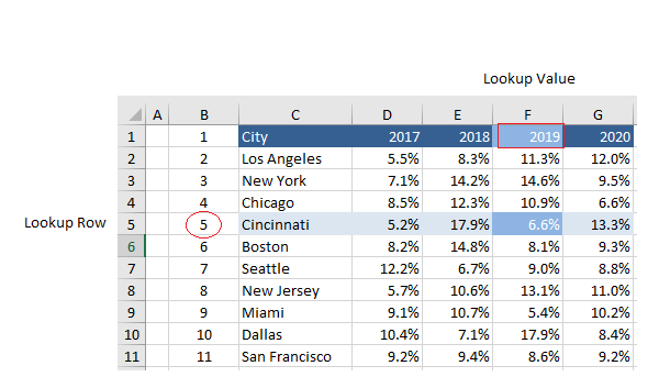
Probably the most well known and used method for HLOOKUP is the exact match. This type of match is ideal especially when you are looking up a unique key and want to return data based on that key. In the following example we will look for 2019 data for the city of Cincinnati.

Once you have identified your unique identifier (2019) you can look up any ROW below the column you are searching for.
The ROW Offset is 5 ROWS as Cincinnati is the 5th row down from the first row, remember to include the first ROW in your count.
The syntax to a HLOOKUP for the above would look like the following:
=HLOOKUP( J2, D1:G11, 5, 0)
Where CELL J2 is the Lookup value 2019, the Range Lookup is D1:G11, the row offset is 5 and the type of LOOKUP is an Exact lookup 0 (this can also be FALSE but why type 5 characters when 1 will do).
To return the CITY for the transaction the only thing we would change would be the ROW reference. This would be 5. For example changing from Cincinnati to New Jersey would mean changing the Reference to 8.
Make the City Flexible
To make the city flexible so you don’t have to know the row reference (5 or 8 using Cincinnati or New Jersey as our example) we might want to incorporate a MATCH formula

The formula would be as follows.
=HLOOKUP( J2, D1:G11,MATCH( I2, C1:C11,0),0)
The MATCH will now allow you to type any city and any year in a cell and have the row reference flex to whatever city is typed. The MATCH works as it looks up the Row Number that the city is in. Thus making the city reference flexible.
The following Excel file will help with a couple of examples of HLOOKUP.