
Excel SUMIFS Formula
The Excel SUMIFS Formula has been long requested and it has addressed a pressing need in the spreadsheet space. Traditionally summing on multiple criteria was the world of the SUMPRODUCT formula, the dark art of Array formula or the use of the humble Excel pivot table. Microsoft changed all that with the advent of the SUMIFS equation. It allows people to SUM a single column based on multiple criteria. It is similar to the SUMIF formula but allows more criteria ranges and criteria to be included in the equation. Just like the SUMIF formula the SUMIFS formula supports operators >, <, <>, = and wildcards *,? for partial cell matching.
The following video outlines the SUMIFS formula with practical examples. The following Excel file outlines the examples.
The SUMIFS Syntax
The following is the syntax for the SUMIFS formula:
=SUMIFS (sum range, Criteria range 1, criteria 1, Criteria range 2, criteria 2 ...)
The arguments for the formula can be broken down as follows.
Sum range - The range to be summed, make this the same length, width as the criteria ranges.
Criteria range 1- The first range to evaluate, make this the same length, width as the SUM range.
Criteria 1 - The criteria to use on range 1, make this the same length, width as the SUM range..
Criteria Range 2 - The second range to evaluate, same length/ width
Criteria 2 - The criteria for the second range.
Note: It is worth pointing out that Criteria Range 3 and criteria 3 follow the same pattern as the two previous criteria and are continued for criteria 4, 5… and up to criteria and range combination totalling to 127. This is overkill though so keep the formulas low with criteria in order to optimise Excel speed and function.
A SUMIFS Example
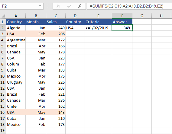
Let’s have a look at a dataset with 2 criteria. We have country and we have month and we want to sum the intersection of USA and January. So the table of data looks as follows.

Column A has the country and column B has the months and column C has the data we want a calculation for or the SUM range. The way this data is structured is perfect for SUMIFS.
The formula to make the calculation is as follows.
=SUMIFS(C2:C19,A2:A19,D2,B2:B19,E2)
The answer to the equation looks as follows:

The SUM range comes first followed by the criteria range and criteria (USA). Criteria range 2 follows with the second criteria (month). This allows the result to be returned which is
223 + 203 = 426
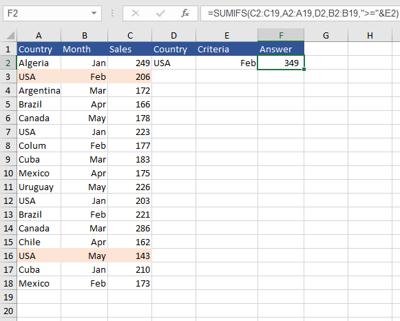
SUMIFS Adding an Operator
If we want to check the dataset for values that are USA for the country and greater than a given month (January) in our data. We can place the operator in the cell or we can hard code the operator in the formula and refer to the cell with the value. Let’s say we want to SUM if the month column is greater than or equal to Feb 19.
The coloured cells are those included in the SUM. Others, which are January, are excluded. It is worth noting that the Months columns are actual Dates not text. It always works better in Excel if we use dates rather than text to represent dates. The syntax becomes:
=SUMIFS(C2:C19,A2:A19,D2,B2:B19,E2)
In the table the >= is added before the date >= 1/02/2019.
Another way to write this formula would be as follows.
=SUMIFS(C2:C19,A2:A19,D2,B2:B19,">="&E2)
In the table the month criteria changes to a regular date.
The attached Excel file has the above examples.
