12 Month Rolling Chart
Creating a rolling 12 month chart in Excel is a valuable interactive tool to add to your spreadsheets. This type of chart will only show 12 months of data and will allow you to scroll forward or backwards in time. The following rolling 12 month chart uses a scroll bar to move the chart between months. There is a small amount of VBA behind the model which will be explained. The rolling 12 month chart can be changed to any length of time by changing the formula associated with the chart.
Here is an example of a 12 month chart that has the scroll bar controlling the chart’s 12 months.
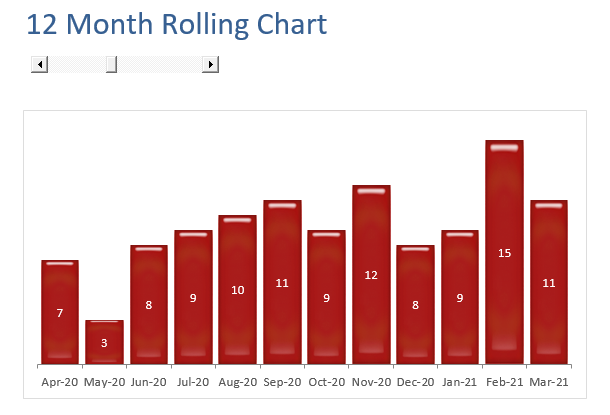
The trick with this chart is to make it dynamic enough to know when there have been new data added to the file. This method will add the new data to the chart’s series as it is entered in the sheet and the scroll bar will recognise the new data as it is added.
Firstly there is a named range called Date;
=OFFSET(Calcs!$A$13,COUNTA(Calcs!$A:$A)+Calcs!$E$10,0,-MIN(12,COUNTA(Calcs!$A:$A)+Calcs!$D$10),1)
Where the amount of months shown in the chart is 12. Just change this number to suit your requirement.
And a second named range called Data;
=Offset(Date,,1)
In E10 I have put the following formula;
=D10-(COUNT(B14:B65)-11)
This formula offsets the rows for the named range Data. It basically ensures that 12 months are only ever shown in the range Data.
and finally in F10 I have put this formula;
=D10-(COUNT(B14:B65)-11)
The formula keeps track of the length of the data and will adjust if new data is added or data is removed ensuring the chart will always show 12 months.
Now add the name range Data to the series in the chart. The following is an example using a screen shot.
Click on the Chart and choose Edit Series.
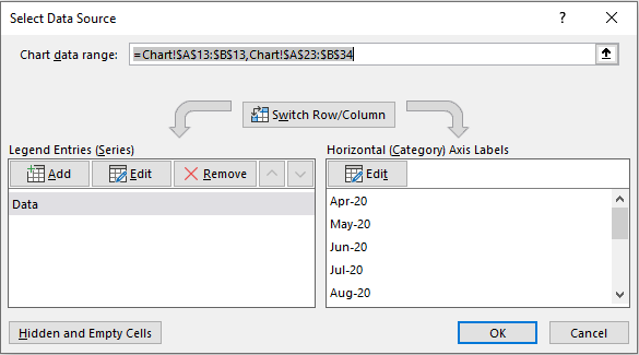
Now click on Edit below Legend Entries Series. Your series values will say something like the following:
=Calcs!$B$14:$B$24
This needs to be changed to;
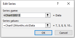
=Calcs!Data
Now the same needs to be done on the right of screen under Horizontal Axis labels click Edit and change.
=Calcs!$B$14:$B$24
Needs to be change to;
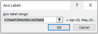
=Calcs!Date
I have inserted an Active X scroll Bar and made D10 the linked cell.
The following is the Excel VBA required to ensure the scroll bar stay up to date when any new data is added. The maximum for the scroll bar needs to be trapped and this is done with 1 line of code and the use of the above formula. It allows the maximum to expand and contract as data is added or removed.
There is a lot to take in above so I have included an Excel file with the formula and VBA coding which should make adapting the file easier.