Lookup Column Value and Header Name

In the following Excel example, I will look up a value on the left and a particular heading and return the value which corresponds to those two criteria (the value and the header).  The traditional use of Vlookup, one of Excel's most widely used and powerful functions, is to lookup a value on the left and return a corresponding value from a table, offset by n Columns to the right.

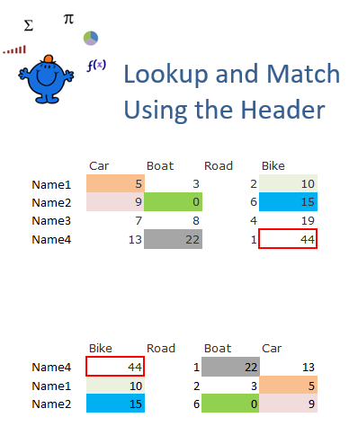
You can see from the table above that the data in the second table (Lookup Table) is jumbled.  The formula in this table is looking up the name on the left, matching that name with a header and returning the corresponding value.  The Excel formula is as follows;
 
=VLOOKUP($B21,$B$11:$F$14,MATCH(C$20,$C$10:$F$10,0)+1,0)

The first part of the formula is looking up the value in B21 - Name4, in B11:F14 - the top table.  Then match is used to match the header in C20 - Bike, with the headings from C10:F10 which are the headers for the top table.
 
I have colour coded the matches and an Excel file is provided to show the workings.  The Excel file should help to crystalise the concept for you.  It is an excellent example of how two nested formula can work together to produce a very nice result.
 
If this article is a little too advanced there is an excellent, groud up article on the VLOOKUP function which concentrates on first principles.  Mikkel and Kasper have taken a concept that may seem foreign and simplified it to create a range of relevant, interesting and practical examples. The article is indepth and very well written and you will glean a great deal from its insights.