
Using an Excel Slicer to Filter Pivot Tables
A slicer is a tool devised in Excel 2010 to isolate items in a pivot table. Slicers work just like the FILTER drop downs on a Pivot Table although they are more visual. Slicers appear on the PivotTable Analyze tab and are associated with both Pivot tables and Excel tables. I mostly use them with a pivot table though.
The following youtube video goes through all of the following and a bit more. File from the video attached below.

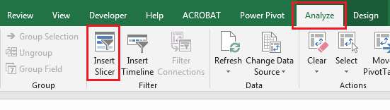
In order to Insert a slicer with a Pivot Table you need to click inside the pivot table.

Click inside the pivot table.
This brings up the Analyze menu.
In the Insert Slicers dialog box, select the check box of the city which is the first item on the list.
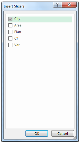
In the above example choose City and click OK.
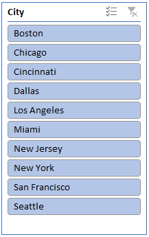
A slicer is displayed for every city that you was in city list The slicer will not filter one, many or all items in the list.
How the Slicer Works
Click on any item in the slicer. HOLD the Ctrl key to select multiple items in the Pivot Table and see how the items are FILTERED inside the Pivot Table. The following is an example.
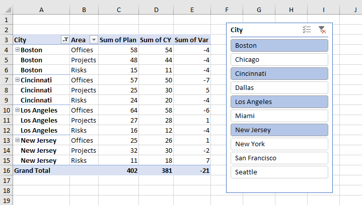
Notice how the items in the slicer replicate the items in the filter. Use the attached Excel file to practice. Enjoy.