
Creating Pivot Tables in Excel
Pivot tables are one of Excel’s powerful features, they allow fast and efficient analysis of large data sets in a small amount of time. Creating Pivot Tables in Excel is a reasonably straight forward process however the structure of the data is most important. If the data is laid out in a tabular format (data in Rows and Columns - no blank fields) then summarising the data becomes a breeze.
The following is the first few lines of the data set we will use to summarise in a Pivot Table.
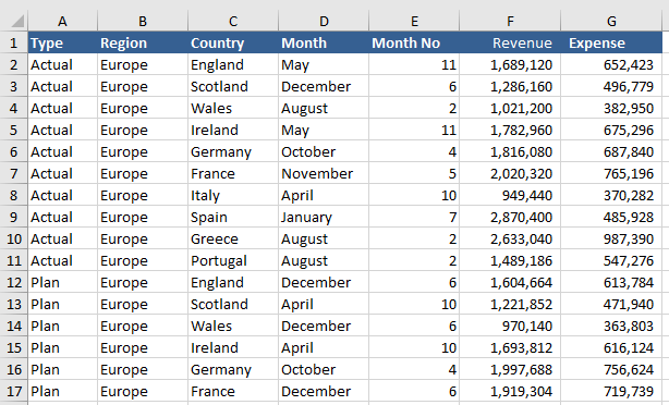
The above is a sample of the data in our workbook. It is financial data that can be sliced and diced a number of ways. It has 7 columns and the data can be split a number of ways. Let’s look at the process of creating a Pivot Table from scratch.
Insert a Pivot Table
Click any cell inside the data set you are working with.
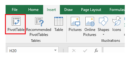
On the Insert Menu Choose - Insert Pivot Table
A dialog will pop up explaining the range of the data set and asking where you want to create the Pivot Table.

The most common place to place a pivot table is a NEW Worksheet. If this is acceptable click OK. Most of my Pivot Tables I put on a fresh sheet.
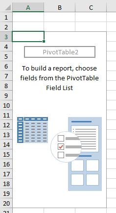
Two menu’s pop up. One is showing you where the Pivot Table will be placed.
And the second dialog showing the fields which can be included in the Pivot Table
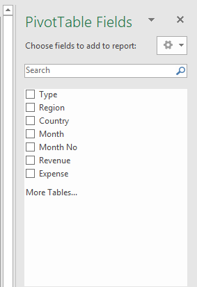
The second dialog on the far right of screen will appear - it shows the fields to add to your Pivot Table.
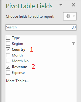
Under Pivot Table Fields choose Country by putting a tick in the box. Then tick Revenue.
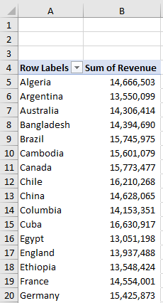
With a few clicks you have a summary by Country by Revenue.
Now add a tick in the Expenses Field.
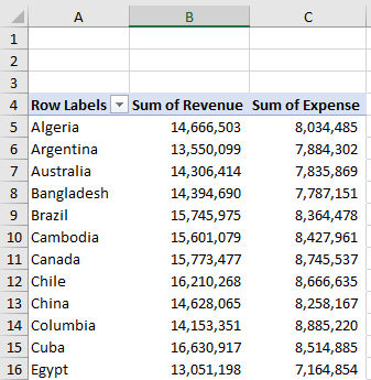
The data instantly gets added to the Pivot Table. The data is now summarised from 600 Row to about 40.
Add A Filter
Filters inside a pivot table are a way of isolating data the same way a Filter in a normal Excel data set would work. They are a great way to summarise data and get instant results in a clear succinct report.
To create a Filter follow the following steps.
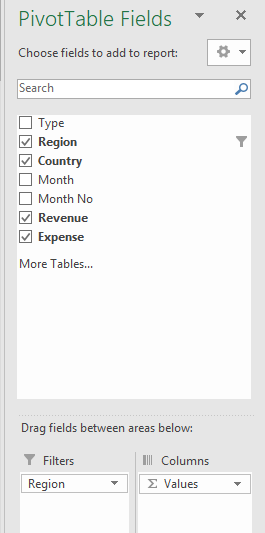
Drag Region down to the Filters section.

On the Pivot Table choose a region from the drop down.
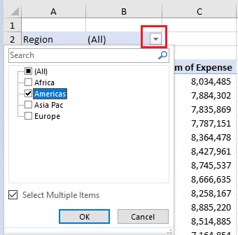
The data will be filtered by the Americas Region.

The data is neatly summarised and you can create further summaries by whatever region you choose. The following file should help which has this data and the completed Pivot Table.