Sum YTD Data
Creating year to date (YTD) comparison based on the current year is a common request in Excel. One of the problems in showing this information is YTD is a moving target. Where March becomes April and so on, so the following question arises, how do we compare current year spend/revenue with last years position? I answered this question on Ozgrid recently where the idea was to update a YTD comparison based on the input for the current year.
The following is a short youtube video on the Excel YTD comparison.
So when you input data into the current month the YTD position for both this year and last are updated. So the update is driven by data entry for this year’s information.
The following is an outline of what the file looks like. It has a full year of data and a part year of data. Our job is to compare them like for like.
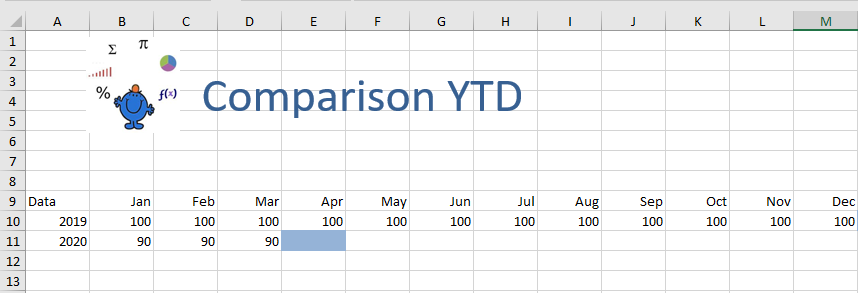
You can see above only 3 months have occurred in the current year. The goal is to compare both years on a like for like basis.
The following is the Excel formula I used.
=SUM(OFFSET($B10:$M10,,,,COUNTA($B11:$M11)))
The Excel formula looks for how many cells in the 2014 dataset are filled. In this case the answer is 3 and the formula to produce that number is;
=SUM(OFFSET($B10:$M10
The last part of the Offset function is Width and if you indicate the range above you can generate the width based on how many cells are produced.
If the starting point is B10 then the offset function is used in conjunction with the CountA formula to offset A9 by 3 columns. The basically counts all of the used cells for the 2014 dataset.
=COUNTA($B11:$M11)
So including B10 the formula will extend 3 columns to produce a rolling YTD result.
The following is a screen shot of the attached Excel file. I have simplified the figures so you can se e the workings.
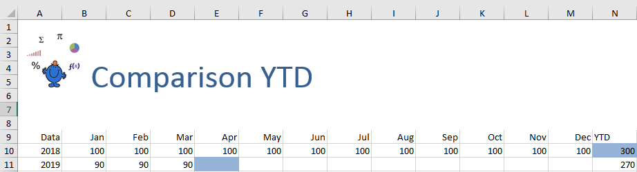
have cells which are filled so only calculates the YTD sum for those three months. The following Excel file shows the above technique.