Creating Dynamic Charts without VBA

The dynamic chart is a fantastic option in Excel. It allows you to create rolling charts and show a variable amount of data at once without doing anything to the chart itself. Without the dynamism of these types of charts every time you need to update your chart you will have to go into its Source Data and change it. The first demonstration will be of a chart which updates with the assistance of Dynamic Ranges.

You can see from some of the Dashboard examples that a well set up data structure does not even need dynamic ranges to create dynamic charts.  Just the intelligent use of the NA() function and offset is a quick and easy work around.  Nonetheless what you need to do is set up a dynamic range for the number of periods you want to show.  In the example I have called this xLen, for the Length of the X Axis.  The formula is as follows;

=OFFSET(Table!$A$1,COUNTA(Table!$A:$A)-1,0,-MIN(n,COUNTA(Table!$A:$A)-1),1)

Where n is a named range, in the file pointing to=ChartVBA!$A$11 which contains the number 10.  So 10 days will be charted.  Changing this value will in turn change the number of days charted.

As there are two series I have added two additional named ranges;

Carlton - 

=OFFSET(xLen,0,1)

Collingwood;

=OFFSET(xLen,0,2)

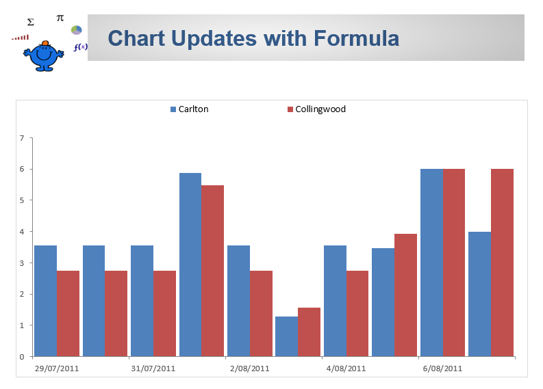
These two named ranges are Series 1 and Series 2 in the chart above.  Now all that is required is for you to change the chart Axis and series to equal these named ranges.  Let’s change the series first.

First, right click on the Excel chart;

Click on the Select data option.

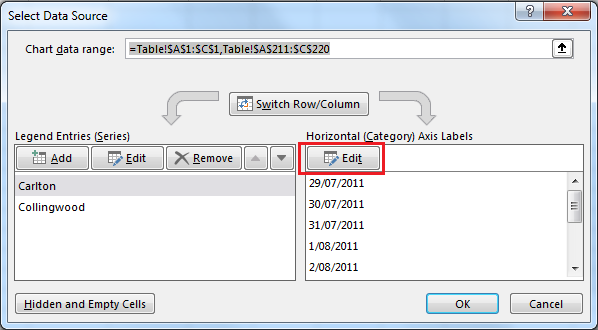
Click on the Edit button as shown above.

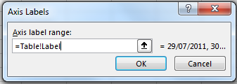
Under the Axis Label Range: Ensure you have the sheet name followed by an exclamation mark.

Table!

now introduce the named range to the end.

Table!xlen

Click OK.  

Follow the same procedure for each of the Series 

Do the same for Series 2 and your chart should be filled with the ranges which are dynamically dependent on an input.

This will show the last 10 days. As you change this number the chart will change in line with the number you type in this cell.

This whole process can be achieved with more complexity by using VBA.  The following is a link to an article which describes this process.

The attached Excel example outlines the above procedure.  It is a simple dynamic Excel chart which should be adaptable for data which is vertical.