
The OFFSET Formula
The Excel OFFSET formula will return a value or text which is Offset from a cell as a starting point. To offset is to move from one position to another and in Excel speak that is exactly what OFFSET does. The Offset formula though has uber functionality as the range can be offset by rows, columns and you can add a height and width to the range which means you can build a range to evaluate which consists of multiple cells. It is often used with rolling forecast or to Sum values based on a number of periods.
The following video takes you through this lesson - file at the bottom of the page. The following Excel file will help to follow along.

The OFFSET Syntax
=OFFSET (Reference, Rows, Cols, Height, Width)
Reference – A cell or range to set the OFFSET formula.
Rows - The amount of rows to OFFSET from the starting point (reference).
Cols - The amount of columns to OFFSET from the starting point (reference).
Height - The height which refers to the rows from the starting point.
Width - The width which refers to the columns from the starting point.
The height and the width are optional which means you don’t have to include them, however the formula takes on the characteristics of the INDEX formula if you are not using the height and width.
OFFSET by Row
Let’s start with the following simple row offset example.
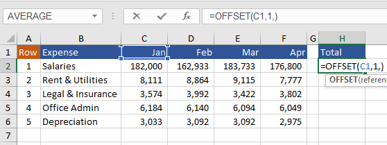
Using the reference in the Offset formula, it starts in C1 the cell (this is the Reference). The ROW offset is 1 which means the OFFSET formula moves one row down and returns the value in C2. The comma at the end is for the column reference and as we are not offsetting by column this is left blank.
=OFFSET(C1,1,)
Note: There needs to be a row and column reference for the OFFSET formula to work.
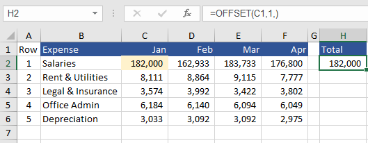
The result is cell C2 = 182K. So we have offset 1 row down.
OFFSET by Column
Let’s have a look at a column offset example with incorporating the row offset above.
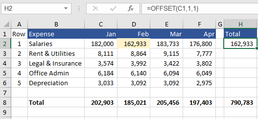
The reference in the above example is the same in C1. The row offset is 1 and the column offset is one so like pawns on a chess board we move one cell down and one across to the right.
=OFFSET(C1,1,1)
The result is to return cell D2 which is the number for Feb.
Incorporating The Offset Height
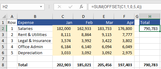
Things get a little tricky when we start to incorporate the height and the width. This is when the result tends to be more than one cell. As a result OFFSET can not return an answer by itself. This is the point where it becomes necessary to nest a formula this is usually a calculation formula. in the following example we will create a sum of a column.

Adding the SUM formula to the equation, we can SUM the values in any given column. As the data is 5 columns deep we will use this is the Height.
=SUM( OFFSET( C1,1,1,5))
The above incorporates the SUM and you can see it is the SUM of February. The reference is C1, offset Row = 1 so the new starting point is C2, then column offset is 1 so the starting point becomes D2, then the height (how many cells to incorporate in the newly created range) is 5. So the range being analysed is D2:D6 which is 5 cells in total.
Incorporating the OFFSET Width
The width relates to widening the range to incorporate more columns. For our example let’s use the entire range of numerical data. The following is the example. The coloured cells are what is being evaluated in the OFFSET formula.
The OFFSET formula becomes.
=SUM(OFFSET(C1,1,0,5,4))
Starting in C1, we move down 1 row and offset no columns (0), then 5 rows deep and 4 columns for the width.
The attached Excel file has the OFFSET formula and the above examples.
