I was recently asked to create a rolling count over more than 40 sheets which were set up as a template - all the same. My first thought was to put a start and end sheet over the workbook and create a Countifs between the start and end tabs. In theory it would work but sadly in practice it was not to be. My next thought was perhaps the indirect function with a list of sheets inside the count area. It proved to be more fruitful. The indirect function is a useful tool if you know how to use it. A formula in a cell:
=Summary!A5
The above is the way that Excel looks at the value in Cell A5 of the Summary sheet. But the following:
=INDIRECT("Summary!A5")
Will produce exactly the same result.
So to my problem: Firstly set your workbook up so you have a list of the sheet names in a column. Your formula has to be the exact same length as the range these cells live in. So no cheating to include extra rows.
=SUMPRODUCT(COUNTIFS(INDIRECT("'"&$N$2:$N$46&"'!"&$A3), ">"&0,INDIRECT("'"&$N$2:$N$46&"'!"&$A3),"<"&5))
The above looks menacing but is simple if you break it down. I would have thought the Countifs function would have been able to get over the line here by itself but it needs the Sumproduct formula to get over the line.
My Sheet tab names are stored from N2:N46 in the sheet I am creating the summary calculation. So be conscious of the cells you put the sheet names in.
The Countifs is performing a calc which says I want the count of all cells greater than zero and less than 5. Where the cell value is in Cell A3.
This should help with this problem. Hope you find it useful.