Excel

TheSmallman.com

an XL ideas Lab

Dashboards VBA
  • Home
  • Dashboards
    • Tips & Tricks
    • Charts
    • Modelling
    • Infographics
    • VBA
  • Shop Dashboards
    • Power Pivot a User Guide
    • Excel Dashboard Course
    • Advanced Dashboard Course
    • Financial Modelling Course
    • Excel VBA Course
  • Blog
  • About
Menu

Excel Dashboards VBA

Street Address
City, State, Zip
Phone Number
an XL ideas Lab

Your Custom Text Here

Excel Dashboards VBA

  • Home
  • Dashboards
  • Excel Tips
    • Tips & Tricks
    • Charts
    • Modelling
    • Infographics
    • VBA
  • Shop Dashboards
  • PowerPivot
    • Power Pivot a User Guide
  • Courses
    • Excel Dashboard Course
    • Advanced Dashboard Course
    • Financial Modelling Course
    • Excel VBA Course
  • Blog
  • About

Evaluate and Filter in Harmony

April 4, 2015 Marcus Small

Performing a check on things like the sheet name with the Evaluate method avoids a looping construct. This tutorial show you how it is done.

On my site I talk a great deal about using the autofilter within code to avoid looping.  It makes a lot of sense as a filter can do in one action what a loop can do in many.  It is a lot faster than looping generally speaking and it uses less VBA coding.

I have been recently experimenting with a new method for looping using the evaluate method. I posted the following code on Chandoos site and I think it worked nicely.  

The request was to take all of the data from sheet1 to sheet2 where column D said the word "Yes" .

The following does this quite quickly.

Option Explicit

Sub FilterToNewLocation()
Dim ar As Variant

   If Application.CountIf(Sheet1.Columns(4), "Yes") = 0 Then Exit Sub
      With Sheet1.[a1].CurrentRegion
         ar = Filter(.Parent.Evaluate("transpose(if(" & .Columns(4).Address & _
         "=""Yes"",row(1:" & .Rows.Count & "),char(2)))"), Chr(2), 0)
         ar = Application.Index(.Value, Application.Transpose(ar), [{1,2,3,4}])
      End With
   Sheet2.[A2].Resize(UBound(ar, 1), 4).Value = ar
End Sub

To replicate the procedure, choose the column your criteria is in Column(4) where 4 needs to change.
Choose the criteria - "Yes" changes to your criteria item.

Choose the columns numbers you want to return {1,2,3,4} and place them in the curly brackets.

Make sure the sheet referencing (Sheet code name) from sheet1 (Sheet1) and to sheet (Sheet2) are in line with your dataset.

I will attach and Excel file to show the workings.  Look out for my next blog post which will be the same method just with 2 criteria.

FilterEvaluate.xls

← Move Sheets Based on a List with VBA Bubble Chart in Excel →

Featured Posts

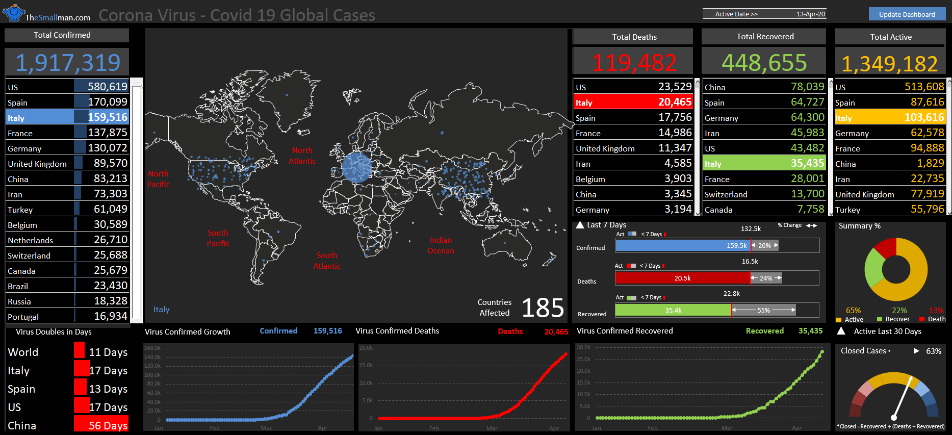
Excel Dashboards: Tracking a Crisis

Excel Dashboards: Tracking a Crisis
April 14, 2020

Recent Posts

Populating an Excel Table from a Range of Cells with VBA

Populating an Excel Table from a Range of Cells with VBA June 12, 2025

Fuzzy Distribution with Randbetween

Fuzzy Distribution with Randbetween May 21, 2025

Add Minimum and Maximum for Chart in Cells

Add Minimum and Maximum for Chart in Cells March 12, 2025

Inflation Over Multiple Years in a Single Cell

Inflation Over Multiple Years in a Single Cell January 10, 2025

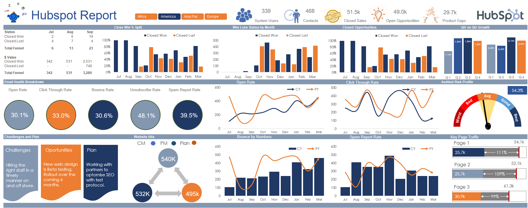
Hubspot Dashboard

Hubspot Dashboard October 3, 2024

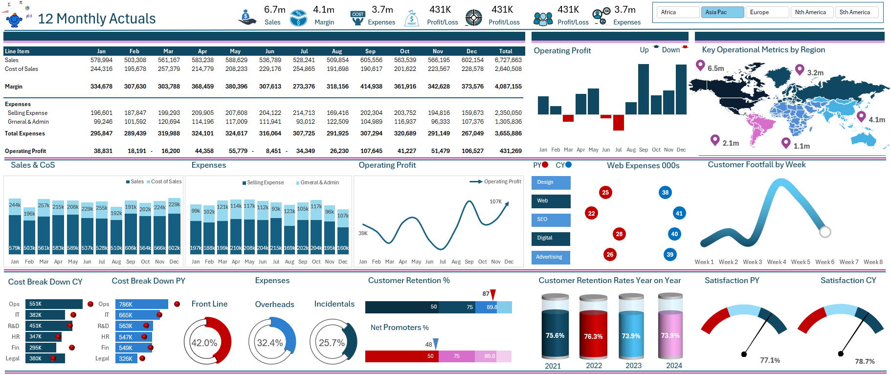
Monthly Dashboard With Supporting Metrics

Monthly Dashboard With Supporting Metrics September 25, 2024

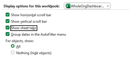
Excel Show Missing Sheet Tabs

Excel Show Missing Sheet Tabs July 29, 2024

Run Macro Overnight Automatically

Run Macro Overnight Automatically June 24, 2024

Split File into Parts and Save to Directory

Split File into Parts and Save to Directory April 20, 2024

Most Popular Author

Most Popular Author December 14, 2023


Follow US:


MarcusSmall@thesmallman.com


TheSmallman.com - Making your small systems hum...
© Copyright 2013-2024 theSmallman.com All Rights Reserved.