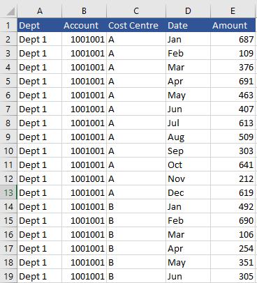
With the advent of Power Pivot the task of flipping data is made very simple. The Unpivot Other Columns command is a bit of a game changer. It easily moves data from horizontal to the more database friendly vertical range very nicely. For the more old school amongst us here is the same task done with VBA. I touched on the opposite of this process in the article Convert Vertical Range to Horizontal with VBA. The following is a common requirement where you have the months in many columns and need to move them to a single column while retaining all of the descriptive information in the report. The following is a sample of what I am talking about.
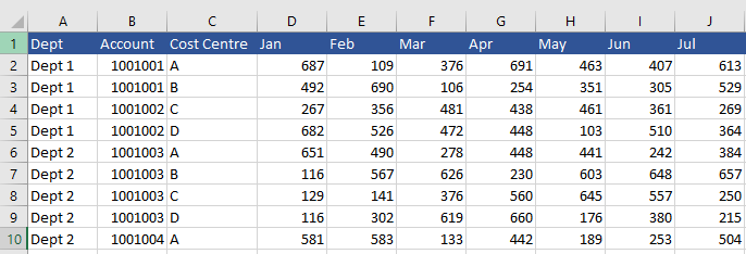
The data is displayed with descriptive information regarding department, account and cost centre while the monthly data is in many columns. What we would like to see is the data on the left 3 columns repeat, while the financial data is repeated row by row. The data output would look as follows.
Notice how now Jan has its own line and Feb has its own line? While the data for dept, account and cost centre repeat? This is a tabular dataset which is a lot easier to work with inside of a database like PowerBi.
The VBA Procedure
How do we spin this data on its head like the above. Well with a simple VBA procedure that I will talk you through. Firstly we need two arrays. One will hold the original data and the other will place the newly formatted data inside.
Option Explicit

Sub Transpose()
Dim ws As Worksheet
Dim sh As Worksheet
Dim ar
Dim var()
Dim i As Long
Dim n As Long
Dim k As Integer
Dim j As Integer
Dim Col as Integer

    Set ws = Sheet1 'Original Data
    Set sh = Sheet2 'Result Sheet
    sh.[A1].CurrentRegion.Offset(1).ClearContents
    ar = ws.UsedRange
    Col = 5 'The total output file columns

    For i = 2 To UBound(ar, 1)
        For j = 4 To 15 'These are the 12 Cols going into 1
            n = n + 1 'Counter
            ReDim Preserve var(1 To Col, 1 To n)
            For k = 1 To 3 'These are the 3 cols that repeat
                var(k, n) = ar(i, k)
            Next k
           var(4, n) = ar(1, j) 'Col 4 is the Date
           var(Col, n) = ar(i, j) 'Monthly Data
        Next j
    Next i
sh.[A2].Resize(n, Col) = WorksheetFunction.Transpose(var)
End Sub
There are two sheets in the workbook - Data tab and an Output tab. These are worksheet code names Sheet1 and Sheet2.
The first array variant is called (ar) this array stores the data in many columns. It picks up the used range
ar = ws.UsedRange
All of data in the Data tab is stored in a the variable and it pretty much happens instantly.
After this point it is a matter of looping through the 15 columns (3 descriptive columns and 12 numerical columns). We turn these 15 column in the ar variant into a 5 column dataset in the output variant (var) and then we output the data to the Output sheet.
For i = 2 To UBound(ar, 1)
The original loop starts from row 2 as we ignore the headings, the headings for the 5 columns are in row 1 of the Output tab. The ubound statement stands for Upper Bound and it is the amount of rows in the variable ar - there are 10 rows in the dataset so it loops from 2 to 10. The first row contains the headings which we ignore.
Turn the Numbers from Horizontal to Vertical
The following is the loop to flip the numbers vertical. So column 4 becomes row 2 column 5 becomes row 3 etc.
For j = 4 To 15
This is column 4 (Jan) to Col 15 (Dec).
The next 2 lines are our counter and the statement that makes our variant (var) dynamic.
n = n + 1
ReDim Preserve var(1 To Col, 1 To n)
The Col is a declared variable this is the total columns in the final output. In the above example Col = 5, so 5 total columns. The n in the first line is a counter, just a way to keep track of the row we want to put the data on. The ReDim line is where the dynamic magic happens. It is saying that the variant (var) is going to be 5 columns in width and will run from 1 to however long the list n is represented so a 5 X n tables where 5 represents the columns and n is the length of those columns.
Repeating the Same Data
The following is the looping construct for the data we want to repeat for each of the 12 months. This will be the department, account and cost centre.
For k = 1 To 3
var(k, n) = ar(i, k)
Next k
The loop starts in column 1 and goes to column 3. This process makes the var equal to what is in the array (ar), in this case that will be ar(2, 1) represented by ar(i,k). The variable in the very first instance i will equal 2 so ar(i = ar(2 and the variable for k in the first instance will be equal to 1 ar(2, 1) where 1 is k on the first part of the loop as the loop goes from 1 to 3 the columns will shift from Column 1 to 2 to 3 while the row will remain the same at 2. As a result row 2 will be filled with the Dept, Account and Cost Centre data with this simple loop.
Adding the Date and Amounts
The following should be the difficult part but as the data is static in terms of the columns then this part is quite straight forward.
var(4, n) = ar(1, j) 'Date
Looking at the date and converting it from row 1 to all of the other rows. The first part of our variant (var) is equal to var(4, n) where 4 is the column number where the date will go and n is the row number which will grow from 2 to the bottom of the range. The reference to our array variant ar is ar(1, j) where 1 is the row and the column is j which is represented by columns 4 to 15. The loop will start at 4 and iterate 1 each loop till it gets to 15.
The second part is to add the amounts to column 5.
var(5, n) = ar(i, j) 'Monthly Data
The var(5, n) is the 5th column and the nth row. The n will grow row by row as with each iteration of the i loop the line.
n = n + 1
appears. This says n is equal to itself plus 1. In the first instance this is 1 then with every iteration of the i loop it will grow by 1. The array ar(i, j) is simply a reference to the row i and the column j that are growing with each iteration of the two loops i and j.
Outputting the Variable to a Range
The procedure is pretty much complete after all the loops have been run. It is a process that runs remarkably quickly. The final step is to transpose the data.
sh.[A2].Resize(n, 5) = WorksheetFunction.Transpose(var)
The above is saying start in row 2 and resize the range to be whatever n landed on so it may be 108 rows and there are 5 columns. The variable (var) gets transposed into that range.
Conclusion and file
Line by line this is effectively how the process is run. If you are running your own dataset and the number of columns vary, just be aware in the test file columns 4 to 15 are being flipped from horizontal to vertical and you can find that in the code. Columns 1 to 3 are staying the same and you can find a reference to this. The final output is going to be 5 columns so work out how many columns you want your output and change this too. Be aware that in my example column 4 is where I put the dates. Find any reference to 4 and change to suit. All the very best. Here is the file to help you with the coding.